

|
|||||||||||||||||||||||||||||||||||||||||||||||||||||||||||||||||||||||||||||||||||||||||||||||||||||||||||||||||||||||||||||||||||||||||||||||||||||||||||||||||||||||||||||||||||||||||||||||||||||||||||||||||||||||||||||||||||||||||||||||||||||||||||||||||||||||||||||||||||||||||||
| Deterministic | Meteorological grid ensemble | Deterministic | |||||||||||||
|---|---|---|---|---|---|---|---|---|---|---|---|---|---|---|---|
| Source: mass estimated from eruption height | Source: mass estimated from eruption height | Source: ESP spreadsheet | |||||||||||||
| Concentrations (1-hour average) | Particles (instantaneous) | Number of members with conc>0 | 90th percentile | Probability of exceeding | |||||||||||
| VAAC | VOLCANO, from Smithsonian | forecast hour | animation | forecast hour | animation | forecast hour | animation | forecast hour | animation | forecast hour | animation | Stamp (ensemble member) plots | Run specifications | scale | forecast hour |
| anchorage | CLEVELAND | loop | loop | loop | loop | loop | txt | ||||||||
| anchorage | SEMISOPOCHNOI | loop | loop | loop | loop | loop | txt | ||||||||
| anchorage | VENIAMINOF | loop | loop | loop | loop | loop | txt | ||||||||
| tokyo | BEZYMIANNY | loop | loop | loop | loop | loop | txt | ||||||||
| tokyo | KARYMSKY | loop | loop | loop | loop | loop | txt | ||||||||
| tokyo | SHIVELUCH | loop | loop | loop | loop | loop | txt | ||||||||
| washington | FUEGO | loop | loop | loop | loop | loop | txt | ||||||||
| washington | KILAUEA | loop | loop | loop | loop | loop | txt | ||||||||
| washington | POPOCATEPETL | loop | loop | loop | loop | loop | txt | ||||||||
| washington | REVENTADOR | loop | loop | loop | loop | loop | txt | ||||||||
| washington | SOUFRIERE_HILLS | loop | loop | loop | loop | loop | txt | ||||||||
| washington | TURRIALBA | loop | loop | loop | loop | loop | txt | ||||||||
If one of these volcanoes has erupted, do not use the charts above; see the products from the appropriate VAAC
These charts are for planning purposes only.
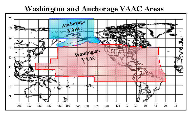
The table above contains volcanoes in and near the Washington and Anchorage VAACs' area of responsibility. The charts are updated four times a day whether the volcanoes have erupted or not. Because the three runs are created separately, if comparisons are made between them, please verify they have the same eruption date/time.
The time of the hypothetical eruption of ash (not SO2) is twelve hours after the initialization time of the NCEP forecast. The forecast duration is 18-hours. The output is one-hourly averaged concentration every 6 hours. For Runs 1 and 2, the ash column top (12192 m = 40,000 ft) and eruption duration (1 hour) are arbitrary; for Run 3, the column top and duration are not arbitrary.
Run 1 produces deterministic dispersion output using a mass eruption rate estimated from the eruption height (Mastin et al., 2009a: A multidisciplinary effort to assign realistic source parameters to models of volcanic ash-cloud transport and dispersion during eruptions, Journal of Volcanology and Geothermal Research, Vol. 186, 10-21), including an estimate of the mass fraction of fine ash. Run 2 uses the same mass eruption rate as in Run 1, but it is an ensemble of 27 members; results from the 27 individual members, are shown, as well as probabilistic ensemble output. The ensemble results are from the HYSPLIT meteorological grid ensemble, not from using any of the NCEP meteorology ensembles. Run 3 produces the dispersion output using the eruption source parameters (ESP) defined by the USGS (Mastin et al., 2009b).
There is always uncertainty in forecasting volcanic ash dispersion in real-time. Basic model inputs such as ash column top height and eruption duration (start and stop time) may or may not be known well. The mass of ash in the eruption is uncertain. The uncertainties of three-dimensional meteorological data (winds, etc.) depend on the meteorological observations used to initialize the model, and the numerical analysis and forecast. An individual model run does not portray any of the model input uncertainty; however, the output for Runs 2 and 3 in this table span some of the input uncertainty and may be useful in interpreting the output from Run 1.
More information on Runs 1, 2, and 3 are given below.
Run 1 produces deterministic dispersion output using a mass eruption rate estimated from the eruption height (Mastin et al., 2009a:, A multidisciplinary effort to assign realistic source parameters to models of volcanic ash-cloud transport and dispersion during eruptions, Journal of Volcanology and Geothermal Research, Vol. 186, 10-21). Briefly, a best-fit line through many historical eruptions showed that H=2.0V^0.241, where H is in km and V in cubic meters dense rock equivalent per second. Assuming a magma density, and a fraction of fine ash that generally remains aloft, we can calculate the mass eruption rate, for input to HYSPLIT, given the eruption height. The best-fit line contains a large amount of scatter due to many factors including uncertainty in estimated ash column height, estimated volumetric eruption rate, temporal variations in eruption height and/or volume, water vapor entrainment, and effect of wind.
Output from the deterministic run is also shown as particle plots, color-coded by height, including a vertical cross section of the plume as viewed perpendicular to the dashed line. These are instantaneous plots, compared to the 1-hour average of the concentration plots.
Run 2 uses an eruption mass estimated from the eruption height. Use of This ensemble is one way to account for some uncertainty in the meteorological model output that is input to the dispersion model. The meteorological ensemble is described here (Draxler, R.R. 2003, Evaluation of an ensemble dispersion calculation, Journal of Applied Meteorology, Vol. 42, February, 308-317). In brief each member of the ensemble is computed by assuming a plus or minus 1-gridpoint shift in the horizontal, and a plus or minus 1500 m shift in the vertical, of the particle position, with respect to the meteorological grid. For the volcanic ash application the vertical shift is much larger than that in the Draxler (2003) because of the generally smaller variability in winds at the higher altitudes than the lower altitudes. The ensemble contains 27 members, including the baseline "control" member with no shift in the particle position. Post-processing sorts the 27 concentrations in ascending order at each concentration grid point. The five types of ensemble output given in the table above are:
This ensemble output can be used in several ways. For example, the animation of the number of members with concentration greater than zero shows the degree of variability among the 27 members. The yellow area is the region where at least 15 members have the ash cloud. The larger this area, the less the uncertainty in the meteorological forecast, and vice versa.
Run 3 is actually several separate model runs. The USGS Volcano Hazards Program has assigned one of 11 eruption types to the world's volcanoes based on recent history. The assigned types are the most likely anticipated future eruption. The USGS also identified eruption source parameters (ESP) for each of these eruption types. The parameters are eruption height, duration, mass flow rate, volume of erupted material and mass fraction of fine ash particles. When these ESP are used, the model output concentration is the actual forecast concentration since an ash mass is input, unlike the unit mass source runs. Excluding the one type for submarine volcanoes, the two main classes of eruption types are defined by magma type (M, mafic; or S, silicic). Then these are classified by general scale ("standard": M0/S0, which is the same as M2/S2; "small": M1/S1, "medium": M2/S2, and "large": M3/S3) or other possible geological effects (pyroclastic flow or "co-ignimbrite cloud" - S8, and "lava dome [collapse]" called "brief": S9). Due to the uncertainties in the ESP by the scale within each mafic of silicic categorization, the output from several eruption scales should be considered for planning purposes. For more information see the report: "Mastin, L.G., Guffanti, M., Ewert, J.E., and Spiegel, J., 2009, Preliminary spreadsheet of eruption source parameters for volcanoes of the world: U.S. Geological Survey Open-File Report 2009-1133, v. 1.2, 25 p."
One way to use this is to look at the ESP forecast hour plot at a given time. If there is an eruption, starting at the given time, and it is has the characteristics of ESP-small, the plume will be as shown for S1/M1. If it has the characteristics of the ESP-large eruption, the plume will be as shown for S3/M3. Then see the time series output using the appropriate ESP-scale link. The ESP classification for the particular run is given in the title at the top of the charts and again at the bottom. Also at the top is given the assigned value. Note that the "brief" category does not pertain to some volcanoes, and the values of the concentration contour lines and the map domains may vary among the various eruption scales.
Inquiries should be addressed to:
Alice Crawford
Email: alice.crawford@noaa.gov
 Volcanic ash (not SO2) cloud forecasts for hypothetical eruptions
